The Figure Shows Two Parallel Nonconducting Rings
News Leon
Mar 18, 2025 · 6 min read
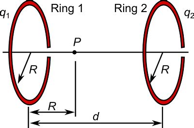
Table of Contents
Exploring the Electric Field of Two Parallel Nonconducting Rings: A Deep Dive
The image depicting two parallel nonconducting rings immediately evokes questions regarding their combined electric field. This seemingly simple scenario offers a rich opportunity to delve into the intricacies of electrostatics, requiring a solid understanding of Coulomb's law, superposition, and integration techniques. This article will comprehensively explore the electric field generated by this configuration, examining various scenarios, simplifying assumptions, and their implications. We will also touch upon potential applications and further extensions of this problem.
Understanding the Fundamentals: Single Ring Electric Field
Before tackling the two-ring system, let's establish a firm grasp of the electric field generated by a single, uniformly charged nonconducting ring. Consider a ring of radius R carrying a total charge Q distributed uniformly along its circumference. To determine the electric field at a point P located on the axis of the ring at a distance z from its center, we employ Coulomb's law and the principle of superposition.
Each infinitesimal charge element dq on the ring contributes a small electric field vector dE at point P. Due to the symmetry of the ring, the components of dE perpendicular to the axis cancel out. Only the axial components remain, and we can integrate these components to find the total electric field. This leads to the well-known expression:
E<sub>z</sub> = (kQz) / (z² + R²)<sup>3/2</sup>
where k is Coulomb's constant (approximately 8.98755 × 10⁹ N⋅m²/C²).
This equation reveals several key features:
- Axial Symmetry: The electric field is directed along the axis of the ring.
- Distance Dependence: The field strength decreases with increasing distance z. At very large distances (z >> R), the field approximates a point charge field (E ≈ kQ/z²).
- Maximum Field: The field is maximized at a specific distance from the ring's center, a detail that becomes crucial when dealing with multiple rings.
Two Parallel Rings: The Superposition Principle
Now, let's consider the scenario of two identical parallel nonconducting rings, each with radius R and charge Q, separated by a distance d. To find the electric field at any point in space, we apply the principle of superposition: the total electric field is the vector sum of the electric fields produced by each ring individually.
This is where the complexity arises. While calculating the field along the common axis connecting the centers of the rings is relatively straightforward (a simple summation of the individual axial fields), determining the field at off-axis points requires more involved calculations. This necessitates the use of vector addition and potentially complex integration techniques depending on the chosen coordinate system.
Calculating the Electric Field along the Common Axis
Let's focus on the electric field along the axis connecting the centers of the two rings. Consider a point P on this axis at a distance z from the center of one ring and z + d from the center of the other. The axial electric field due to each ring can be calculated using the equation derived earlier. The total electric field at P is simply the sum of the two individual fields:
E<sub>total</sub> = E<sub>ring1</sub> + E<sub>ring2</sub>
E<sub>total</sub> = (kQz) / (z² + R²)<sup>3/2</sup> + (kQ(z+d)) / ((z+d)² + R²)<sup>3/2</sup>
This equation provides the electric field at any point along the common axis. Analyzing this equation reveals that:
- Zero Field Point: Depending on the values of R and d, there might exist a point along the axis where the electric field becomes zero. This occurs when the electric fields from each ring exactly cancel each other out.
- Field Strength Variations: The field strength varies significantly along the axis, depending on the distance from each ring. Regions of strong and weak fields can exist depending on the ring's spacing and charge.
- Approximations: For large distances (z >> R, z >> d), the total field approaches the field of two point charges separated by d.
Off-Axis Electric Field Calculation: A Challenging Task
Calculating the electric field at points off the common axis is significantly more challenging. The simplicity of axial symmetry is lost, and we must consider both the x and y components of the electric field vectors contributed by each ring. This typically involves integration in a polar or Cartesian coordinate system, taking into account the varying distance and angle between each charge element and the point of interest. Analytical solutions for arbitrary points are often intractable, necessitating numerical methods or approximations.
Simplifying Assumptions and Approximations
To facilitate calculations, several simplifying assumptions can be made:
- Large Distance Approximation: If the distance from the rings is much greater than their radii (z >> R, d >> R), we can approximate each ring as a point charge. This significantly simplifies the calculations.
- Small Separation Approximation: If the separation between the rings is much smaller than their radii (d << R), the system can be treated as a continuous charge distribution, potentially simplifying the problem to a different geometry.
- Numerical Methods: For complex scenarios, numerical methods such as finite element analysis (FEA) or boundary element methods (BEM) can be used to approximate the electric field.
Applications and Extensions
Understanding the electric field of parallel rings has applications in various areas:
- Electrostatic Lenses: Arrays of charged rings can be used to create electrostatic lenses for focusing charged particles in electron microscopes or other scientific instruments. The field’s complex behavior influences beam shaping and focusing capabilities.
- Antenna Design: The radiation patterns of antennas can be analyzed using similar principles, where the rings represent different parts of the antenna structure.
- Modeling Charge Distributions: This problem serves as a fundamental example for studying more complex charge distributions.
- Electrostatic Traps: The carefully designed electric fields from parallel rings can be used to trap charged particles in a confined region.
Conclusion
The problem of two parallel nonconducting rings, while seemingly straightforward, offers a compelling exploration of electrostatics and its complexities. While calculating the electric field along the common axis is relatively manageable, calculating the off-axis field necessitates more advanced techniques. Various approximations and numerical methods can be utilized to address the complexity, providing insights into the system's behavior. This comprehensive analysis highlights the importance of understanding superposition, symmetry, and integration techniques in electrostatics, and its relevance extends to several fields of physics and engineering. Further research could explore the effect of different charge distributions on the rings, the impact of varying ring radii, and optimization strategies for achieving specific electric field profiles.
Latest Posts
Latest Posts
-
1 1 2 4 3 9 4
Mar 19, 2025
-
Oxidation Number Of S In H2so4
Mar 19, 2025
-
In Meiosis Homologous Chromosomes Separate During
Mar 19, 2025
-
What Is A Polymer For Lipids
Mar 19, 2025
-
Why Is Boiling Water A Physical Change
Mar 19, 2025
Related Post
Thank you for visiting our website which covers about The Figure Shows Two Parallel Nonconducting Rings . We hope the information provided has been useful to you. Feel free to contact us if you have any questions or need further assistance. See you next time and don't miss to bookmark.
