The Figure Shows Two Charged Particles On An X Axis
News Leon
Mar 15, 2025 · 6 min read
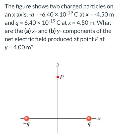
Table of Contents
The Figure Shows Two Charged Particles on an X-Axis: A Deep Dive into Electrostatics
This article delves into the fascinating world of electrostatics, specifically focusing on the interaction of two charged particles positioned on the x-axis. We'll explore the fundamental concepts, delve into the calculations involved in determining the net electric field and potential, and examine how these principles apply to more complex scenarios. This exploration will be rich with examples and explanations to build a strong intuitive understanding.
Understanding the Fundamentals: Charge and Coulomb's Law
At the heart of this discussion lies Coulomb's Law, the cornerstone of electrostatics. This law quantifies the force between two point charges, stating that the force is directly proportional to the product of the charges and inversely proportional to the square of the distance separating them. Mathematically, this is represented as:
F = k * |q1 * q2| / r²
Where:
- F represents the electrostatic force (in Newtons).
- k is Coulomb's constant (approximately 8.98755 × 10⁹ N⋅m²/C²).
- q1 and q2 are the magnitudes of the two charges (in Coulombs).
- r is the distance between the charges (in meters).
The direction of the force is along the line connecting the two charges. Like charges (both positive or both negative) repel each other, resulting in a positive force, while opposite charges attract, leading to a negative force (though the magnitude of the force is still positive). This seemingly simple equation unlocks a universe of electrostatic phenomena.
Analyzing Two Charges on the X-Axis: A Step-by-Step Approach
Let's consider a specific scenario: two charged particles, q1 and q2, are located on the x-axis at positions x1 and x2, respectively. We can systematically analyze the electric field and potential at various points along the x-axis and beyond.
Calculating the Electric Field
The electric field at a point in space is defined as the force per unit charge experienced by a small positive test charge placed at that point. To find the net electric field (E) at a point x on the x-axis due to q1 and q2, we need to consider the individual contributions from each charge and then sum them vectorially.
- Electric Field due to q1: The magnitude of the electric field due to q1 at point x is given by:
E1 = k * |q1| / (x - x1)²
The direction is determined by the sign of q1 and the relative position of x and x1. If x > x1 and q1 is positive, the field points in the positive x-direction; if x < x1 and q1 is positive, the field points in the negative x-direction, and so on.
- Electric Field due to q2: Similarly, the magnitude of the electric field due to q2 at point x is:
E2 = k * |q2| / (x - x2)²
The direction is determined by the sign of q2 and the relative positions of x and x2.
- Net Electric Field: The net electric field at point x is the vector sum of E1 and E2. Since both fields are along the x-axis, the net field is simply the algebraic sum (considering direction via sign).
E_net = E1 + E2
This calculation becomes particularly important when determining the point(s) where the net electric field is zero. This often involves solving a quadratic equation.
Calculating the Electric Potential
Electric potential (V) is a scalar quantity that represents the electric potential energy per unit charge at a point in space. The potential at a point x due to a single point charge q is:
V = k * q / r
where r is the distance from the charge to the point.
For our two-charge system on the x-axis, the total potential at point x is the scalar sum of the potentials due to each charge:
V_net = V1 + V2 = k * q1 / (x - x1) + k * q2 / (x - x2)
This calculation is generally simpler than calculating the electric field, as it involves only scalar addition. Finding points where the potential is zero often involves solving a simpler equation compared to finding points of zero electric field.
Extending the Concepts: Beyond the X-Axis
The principles discussed above can be extended to analyze the electric field and potential at points off the x-axis. However, the calculations become more complex, requiring vector addition in two or three dimensions. The individual field components (x, y, z) need to be calculated and then combined using vector addition.
For points not on the x-axis, we use the distance formula to calculate the distance 'r' from each charge to the point of interest. This involves calculating the square root of the sum of the squares of the x, y, and z distances. The direction of the electric field at each point is no longer simply along the x-axis, making the vector summation critical.
Applications and Real-World Examples
Understanding the behavior of two charged particles on an x-axis has numerous applications in various fields:
-
Particle Accelerators: The design and operation of particle accelerators heavily rely on manipulating the electric fields created by strategically placed charged particles to accelerate and guide charged beams.
-
Electronics: The behavior of electrons and other charged particles in electronic circuits can be modeled using the principles of electrostatics. Understanding the interaction of these particles is crucial for designing efficient and reliable electronic devices.
-
Medical Imaging: Techniques like MRI (Magnetic Resonance Imaging) utilize the principles of electromagnetism and the interaction of charged particles to generate detailed images of the human body.
-
Atmospheric Physics: The study of lightning and other atmospheric phenomena involves understanding the interaction of charged particles in the atmosphere.
Solving Advanced Problems: A Practical Example
Let's consider a concrete example. Suppose we have two charges, q1 = +2 µC located at x1 = -1 m and q2 = -3 µC located at x2 = +2 m. Let's find the net electric field and potential at point x = 0 m.
First, we calculate the electric field due to each charge at x = 0:
-
E1 = k * |q1| / (x - x1)² = (8.98755 × 10⁹ N⋅m²/C²) * (2 × 10⁻⁶ C) / (-1 m)² = 1.7975 × 10⁴ N/C (in the positive x-direction)
-
E2 = k * |q2| / (x - x2)² = (8.98755 × 10⁹ N⋅m²/C²) * (3 × 10⁻⁶ C) / (2 m)² = 6.7406 × 10³ N/C (in the negative x-direction)
The net electric field is:
E_net = E1 + E2 = 1.7975 × 10⁴ N/C - 6.7406 × 10³ N/C = 1.1234 × 10⁴ N/C (in the positive x-direction)
Now, let's calculate the potential at x = 0:
-
V1 = k * q1 / (x - x1) = (8.98755 × 10⁹ N⋅m²/C²) * (2 × 10⁻⁶ C) / (-1 m) = -1.7975 × 10⁴ V
-
V2 = k * q2 / (x - x2) = (8.98755 × 10⁹ N⋅m²/C²) * (-3 × 10⁻⁶ C) / (2 m) = -1.3481 × 10⁴ V
The net potential is:
V_net = V1 + V2 = -1.7975 × 10⁴ V - 1.3481 × 10⁴ V = -3.1456 × 10⁴ V
This example demonstrates the practical application of the principles discussed. Remember to always account for the signs of the charges and the directions of the electric fields when performing these calculations.
Conclusion
The seemingly simple scenario of two charged particles on an x-axis provides a rich foundation for understanding the fundamental principles of electrostatics. Through careful application of Coulomb's Law and the concepts of electric field and potential, we can analyze the interaction of these charges and predict their behavior. This understanding extends to a broad range of applications in various scientific and engineering disciplines. This article serves as a starting point for further exploration of the fascinating world of electrostatics and its multifaceted applications. The key is to systematically break down the problem, considering each charge's contribution individually before combining them correctly, accounting for both magnitude and direction.
Latest Posts
Latest Posts
-
Viral Capsids Are Made From Subunits Called
Mar 15, 2025
-
A Negatively Charged Ion Is Called
Mar 15, 2025
-
Two Different Isotopes Of An Element Have Different
Mar 15, 2025
-
If A Pea Plant Shows A Recessive Phenotype
Mar 15, 2025
-
Is A Patent A Current Asset
Mar 15, 2025
Related Post
Thank you for visiting our website which covers about The Figure Shows Two Charged Particles On An X Axis . We hope the information provided has been useful to you. Feel free to contact us if you have any questions or need further assistance. See you next time and don't miss to bookmark.
