How To Calculate Long Run Equilibrium Price
News Leon
Mar 26, 2025 · 6 min read
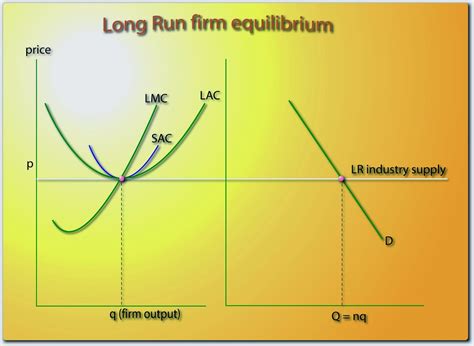
Table of Contents
How to Calculate the Long-Run Equilibrium Price: A Comprehensive Guide
The long-run equilibrium price is a crucial concept in economics, representing the price at which a market settles after all adjustments have been made. Unlike the short-run equilibrium, which might be influenced by temporary supply or demand shocks, the long-run equilibrium reflects a state of stability where firms have optimized their production and consumers have reached their desired consumption levels. Understanding how to calculate this price requires a grasp of market structures and their respective characteristics. This comprehensive guide will walk you through the process, exploring different market models and providing practical examples.
Understanding Market Structures and Their Impact on Long-Run Equilibrium
Before diving into the calculations, it's crucial to understand the various market structures, as each dictates a different approach to determining the long-run equilibrium price.
1. Perfect Competition
Perfect competition is a theoretical market structure characterized by:
- Many buyers and sellers: No single participant can influence the market price.
- Homogenous products: All goods are identical, making them perfect substitutes.
- Free entry and exit: Firms can easily enter or leave the market.
- Perfect information: All participants have complete knowledge of prices and costs.
In perfect competition, the long-run equilibrium price is determined where the average total cost (ATC) curve intersects the demand curve and is equal to the marginal cost (MC) and marginal revenue (MR). This point signifies zero economic profit for firms, as price equals both average total cost and marginal cost. If the price were above this point, new firms would enter the market, increasing supply and driving the price down. Conversely, if the price were below this point, firms would exit, reducing supply and pushing the price up.
In essence, the long-run equilibrium price in perfect competition is the minimum point of the average total cost curve.
2. Monopolistic Competition
Monopolistic competition shares some similarities with perfect competition but also introduces key differences:
- Many buyers and sellers: Similar to perfect competition.
- Differentiated products: Products are similar but not identical, offering some degree of product differentiation.
- Relatively easy entry and exit: Barriers to entry are lower than in a monopoly but higher than in perfect competition.
- Imperfect information: Buyers may not have complete knowledge of all available options.
In monopolistic competition, the long-run equilibrium is achieved where the demand curve is tangent to the average total cost curve. Unlike perfect competition, firms earn zero economic profit but maintain some level of market power due to product differentiation. The price is higher than the marginal cost, reflecting the monopolistic element of the market. This is because firms have some control over price due to product differentiation, although the competition still limits their ability to charge exorbitant prices.
3. Oligopoly
Oligopolies are characterized by:
- Few large firms: A small number of firms dominate the market.
- Homogenous or differentiated products: Products can be either identical or differentiated.
- Significant barriers to entry: High start-up costs or other obstacles prevent new firms from easily entering.
- Interdependence: Firms' decisions are influenced by the actions of their competitors.
Calculating the long-run equilibrium price in an oligopoly is complex and doesn't have a single, universally applicable formula. The outcome heavily depends on the firms' strategies (e.g., collusion, price wars, non-price competition) and the specific market conditions. Game theory is often used to model the interactions between firms and predict potential outcomes. The long-run equilibrium might involve prices above marginal cost, indicating economic profits, especially if firms engage in collusion.
4. Monopoly
Monopolies possess the following characteristics:
- Single seller: Only one firm controls the entire market.
- Unique product: No close substitutes exist.
- High barriers to entry: Significant obstacles prevent new firms from entering.
- Price maker: The monopolist can influence the market price.
In a monopoly, the long-run equilibrium is where the marginal revenue (MR) curve intersects the marginal cost (MC) curve. The monopolist then uses the demand curve to determine the price corresponding to this quantity. This results in a price significantly higher than the marginal cost, and the monopolist earns substantial economic profits. There's no guarantee of efficiency, as the monopolist restricts output to maximize its profit.
Practical Examples and Calculations
Let's illustrate the calculation of the long-run equilibrium price with some simplified examples.
Example 1: Perfect Competition
Imagine a perfectly competitive market for wheat. Suppose the market demand function is given by: P = 100 - 0.5Q, where P is the price and Q is the quantity. The average total cost (ATC) function for a representative firm is: ATC = 20 + 0.1Q + 0.01Q².
In perfect competition, the long-run equilibrium occurs where P = ATC = MC. We need to find the MC function by deriving the ATC function:
MC = d(ATC)/dQ = 0.1 + 0.02Q
We solve for Q where MC = ATC:
0.1 + 0.02Q = 20 + 0.1Q + 0.01Q²
This is a quadratic equation, which when solved (using the quadratic formula or other methods), yields a positive value for Q. Substituting that value of Q back into either the ATC or MC equation gives us the long-run equilibrium price (P).
Example 2: Monopolistic Competition (Simplified)
This example will be simplified due to the complexity inherent in deriving the optimal solution. Let's assume a firm in a monopolistically competitive market has a demand curve given by: P = 50 - Q. Assume the average total cost is a simplified linear function: ATC = 20 + 0.5Q.
To find the long-run equilibrium, we need to find where the demand curve is tangent to the ATC curve. This requires more advanced calculus (finding the point where the slopes of the two curves are equal), which is beyond the scope of a simplified explanation. Graphically, it would be the point where the two curves just touch. Solving this analytically requires setting the derivative of the demand curve equal to the derivative of the ATC curve and solving the resulting system of equations.
Factors Affecting Long-Run Equilibrium Price
Several factors can influence the long-run equilibrium price, even within the same market structure:
- Changes in technology: Technological advancements can lower production costs, shifting the ATC curve downward and potentially lowering the equilibrium price.
- Changes in consumer preferences: A shift in consumer demand will affect the demand curve, impacting the equilibrium price.
- Government regulations: Taxes, subsidies, or price controls can significantly alter the equilibrium price.
- Changes in input prices: Increases in the cost of raw materials or labor can shift the ATC curve upward, leading to a higher equilibrium price.
- Entry and exit of firms: As discussed earlier, the entry and exit of firms play a crucial role in adjusting the supply and ultimately impacting the equilibrium price, particularly in markets with relatively easy entry and exit.
Conclusion
Calculating the long-run equilibrium price is a crucial aspect of economic analysis. The process varies depending on the market structure, ranging from a straightforward solution in perfect competition to complex game-theoretic models in oligopolies. Understanding the factors that influence the long-run equilibrium price allows for better prediction of market behavior and informed decision-making. While simplified examples were used for illustrative purposes, real-world applications often require more sophisticated modeling and data analysis. However, the fundamental principles outlined here provide a solid foundation for understanding this important economic concept. This requires careful consideration of market structure, relevant cost functions, and demand conditions. Remember that the long-run equilibrium represents a state of relative stability, but it's a dynamic equilibrium that constantly adjusts in response to changing market conditions.
Latest Posts
Latest Posts
-
How Much Money Did Kalam Earn After Selling Seeds
Mar 29, 2025
-
Boiling Water Is A Chemical Change
Mar 29, 2025
-
An Oscillating Block Spring System Has A Mechanical Energy
Mar 29, 2025
-
A Manager Who Maintains A Stakeholder View Will
Mar 29, 2025
-
In Which Organelle Does Cellular Respiration Take Place
Mar 29, 2025
Related Post
Thank you for visiting our website which covers about How To Calculate Long Run Equilibrium Price . We hope the information provided has been useful to you. Feel free to contact us if you have any questions or need further assistance. See you next time and don't miss to bookmark.
