How To Find Instantaneous Rate Of Change From A Table
News Leon
Apr 02, 2025 · 8 min read
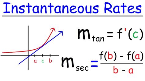
Table of Contents
- How To Find Instantaneous Rate Of Change From A Table
- Table of Contents
- How to Find the Instantaneous Rate of Change from a Table
- Understanding Instantaneous Rate of Change
- Method 1: Using the Secant Line Approximation
- Method 2: Using Numerical Differentiation (Central Difference Method)
- Method 3: Polynomial Interpolation
- Method 4: Spline Interpolation
- Choosing the Right Method
- Software and Tools
- Conclusion
- Latest Posts
- Latest Posts
- Related Post
How to Find the Instantaneous Rate of Change from a Table
Determining the instantaneous rate of change from a table of data points requires a slightly different approach than using a function's equation. Since you don't have a continuous function, you can't directly use derivatives. Instead, we rely on approximations using techniques from calculus. This article will guide you through several methods, focusing on accuracy and practical application.
Understanding Instantaneous Rate of Change
Before diving into the methods, let's clarify the concept. The instantaneous rate of change represents the rate at which a quantity is changing at a specific point in time. Think of it as the slope of the tangent line to a curve at a particular point. In the context of a table, we're essentially estimating the slope of this tangent line using nearby data points.
Method 1: Using the Secant Line Approximation
This is the most straightforward method, albeit the least precise. We approximate the instantaneous rate of change at a point by calculating the average rate of change over a small interval surrounding that point. The smaller the interval, the better the approximation.
Steps:
-
Identify the Point of Interest: Determine the specific x-value (let's call it x<sub>0</sub>) at which you need the instantaneous rate of change.
-
Select Neighboring Points: Choose data points immediately before and after x<sub>0</sub>. Let's call these (x<sub>1</sub>, y<sub>1</sub>) and (x<sub>2</sub>, y<sub>2</sub>), where x<sub>1</sub> < x<sub>0</sub> < x<sub>2</sub>.
-
Calculate the Average Rate of Change: The average rate of change (which approximates the instantaneous rate of change) is given by:
(y<sub>2</sub> - y<sub>1</sub>) / (x<sub>2</sub> - x<sub>1</sub>)
Example:
Let's say we have the following table representing the position of an object over time:
| Time (s) | Position (m) |
|---|---|
| 1 | 2 |
| 2 | 5 |
| 3 | 10 |
| 4 | 17 |
| 5 | 26 |
We want to find the instantaneous rate of change of position (velocity) at t = 3 seconds.
Using the points (2, 5) and (4, 17):
Average rate of change = (17 - 5) / (4 - 2) = 6 m/s
This is an approximation of the instantaneous velocity at t = 3s. A smaller interval would likely provide a more accurate approximation but might not always be possible with the given data.
Limitations: This method's accuracy depends heavily on the spacing of the data points. Closely spaced points yield better approximations. It's also susceptible to noise in the data.
Method 2: Using Numerical Differentiation (Central Difference Method)
The central difference method provides a more refined approximation than the simple secant line method. It leverages data points on both sides of the point of interest to reduce the error associated with one-sided approximations.
Steps:
-
Identify the Point of Interest: Same as before, identify the x-value (x<sub>0</sub>) where you need the instantaneous rate of change.
-
Select Neighboring Points: Select the data point immediately before (x<sub>-1</sub>, y<sub>-1</sub>) and immediately after (x<sub>1</sub>, y<sub>1</sub>) x<sub>0</sub>.
-
Calculate the Central Difference: The central difference approximation of the derivative is:
(y<sub>1</sub> - y<sub>-1</sub>) / (x<sub>1</sub> - x<sub>-1</sub>)
Example:
Using the same table as before, let's approximate the instantaneous velocity at t = 3 seconds using the central difference method.
We'll use points (2, 5) and (4, 17):
Central difference = (17 - 5) / (4 - 2) = 6 m/s
Notice that in this particular example, the central difference yields the same result as the simple secant line method. However, this is not always the case, especially with unevenly spaced data points. The central difference method generally provides a more accurate approximation.
Advantages: The central difference method generally provides a more accurate estimate of the instantaneous rate of change compared to using only one neighboring point. This is because it considers the slope from both sides, averaging out potential errors.
Limitations: Requires at least two data points on either side of the point of interest. Still an approximation and susceptible to noise in the data. Uneven spacing of data points can affect accuracy.
Method 3: Polynomial Interpolation
For more accurate approximations, especially when dealing with unevenly spaced data or when higher accuracy is needed, polynomial interpolation can be a powerful technique. It involves fitting a polynomial function to the data points and then taking the derivative of that polynomial at the desired point.
Steps:
-
Select Relevant Data Points: Choose several data points surrounding x<sub>0</sub>. The more points you use, the higher the degree of the polynomial and potentially the better the approximation (but also the higher the risk of overfitting if data is noisy).
-
Perform Polynomial Interpolation: Several methods exist for polynomial interpolation, including Lagrange interpolation and Newton's divided difference interpolation. These methods find a polynomial that passes exactly through the selected data points. This is computationally more intensive than the previous methods.
-
Differentiate the Polynomial: Once you have the interpolating polynomial, find its derivative.
-
Evaluate the Derivative: Substitute x<sub>0</sub> into the derivative to obtain the approximate instantaneous rate of change.
Example:
Let's consider a simplified example with evenly spaced data for demonstration purposes. Performing polynomial interpolation by hand for complex datasets is challenging and usually requires computational tools like spreadsheets or programming languages (Python with NumPy or SciPy are ideal).
Suppose we have the following data:
| x | y |
|---|---|
| 1 | 1 |
| 2 | 8 |
| 3 | 27 |
| 4 | 64 |
We want to approximate the instantaneous rate of change at x = 2. Using a quadratic interpolation (passing through points (1,1), (2,8), (3,27)), we'd obtain a polynomial, and then we'd differentiate it and evaluate the derivative at x=2 to obtain the approximation.
Advantages: Polynomial interpolation offers greater accuracy than simpler methods, particularly with unevenly spaced data. It can capture more complex patterns in the data.
Limitations: Computationally more intensive. Higher-degree polynomials can be susceptible to overfitting, especially with noisy data. Choosing the appropriate number of data points is crucial. The selection of interpolation method also impacts accuracy.
Method 4: Spline Interpolation
Spline interpolation is a sophisticated technique that extends polynomial interpolation by fitting piecewise polynomial functions to the data. This method avoids the problems of high-degree polynomials oscillating wildly between data points, which is a common issue with polynomial interpolation.
Spline interpolation uses multiple lower-degree polynomials, each defined over a subinterval of the data. This approach often leads to smoother and more accurate approximations of the instantaneous rate of change, especially when dealing with complex curves or noisy data. Cubic splines are commonly used because they offer a good balance between smoothness and computational complexity.
Steps:
-
Divide the Data: Divide the data into intervals.
-
Fit Splines: Fit a low-degree polynomial (usually cubic) to each interval. The polynomials are constrained to have continuous first and second derivatives at the interval boundaries, resulting in a smooth curve.
-
Differentiate the Splines: Find the derivative of each spline.
-
Evaluate at the Point: Evaluate the appropriate spline's derivative at the desired x<sub>0</sub> to obtain the approximate instantaneous rate of change.
Advantages: Smooth, accurate approximations, especially with noisy or unevenly spaced data. Avoids the oscillations of high-degree polynomials.
Limitations: Computationally more intensive than simpler methods. Requires specialized software or programming to implement efficiently.
Choosing the Right Method
The best method for approximating the instantaneous rate of change from a table depends on several factors:
-
Data Spacing: Evenly spaced data simplifies calculations. Uneven spacing often necessitates more sophisticated methods like polynomial or spline interpolation.
-
Data Noise: Noisy data can significantly impact the accuracy of any method. Smoothing techniques or robust methods (like spline interpolation) might be necessary.
-
Accuracy Requirements: For rough estimates, the secant line or central difference methods might suffice. For higher accuracy, polynomial or spline interpolation are preferable.
-
Computational Resources: Simpler methods require less computation, while polynomial and spline interpolation require more computing power and software support.
Software and Tools
While basic methods can be done by hand, more sophisticated approaches like polynomial and spline interpolation typically require computational tools. Spreadsheets (like Excel or Google Sheets) can handle simple interpolations and numerical differentiation. Programming languages like Python (with libraries such as NumPy and SciPy), MATLAB, or R provide powerful tools for implementing these methods effectively and efficiently for larger datasets.
Conclusion
Finding the instantaneous rate of change from a table involves approximating the slope of the tangent line at a specific point using neighboring data points. Several methods exist, ranging from simple average rate of change calculations to more sophisticated techniques like polynomial and spline interpolation. The choice of method should be guided by the characteristics of the data, the required accuracy, and the available computational resources. Remember that any method applied to tabular data will provide only an approximation of the true instantaneous rate of change.
Latest Posts
Latest Posts
-
Boiling Water Is A Physical Or Chemical Change
Apr 05, 2025
-
Which Of The Following Is Not An Oxidation Reduction Reaction
Apr 05, 2025
-
A Scientist That Studies Minerals Is Called A
Apr 05, 2025
-
How Do You Graph X 5
Apr 05, 2025
-
Poor Conductors Of Heat And Electricity
Apr 05, 2025
Related Post
Thank you for visiting our website which covers about How To Find Instantaneous Rate Of Change From A Table . We hope the information provided has been useful to you. Feel free to contact us if you have any questions or need further assistance. See you next time and don't miss to bookmark.
